PyGMT: High-Resolution Topographic Map in Python (codes included)

Introduction

If you have been working in seismology, then you must have come across Generic Mapping Tools (GMT) software. It is widely used software, not only in seismology but across the Earth, Ocean, and Planetary sciences and beyond. It is a free, open-source software used to generate publication quality maps or illustrations, process data and make animations. Recently, GMT built API (Application Programming Interface) for MATLAB, Julia and Python. In this post, we will explore the Python wrapper library for the GMP API - PyGMT. Using the GMT from Python script allows enormous capabilities.

The API reference for PyGMT can be accessed from here and is strongly recommended. Although PyGMT project is still in completion, there are many functionalities available.

Step-by-step guide for PyGMT using an example

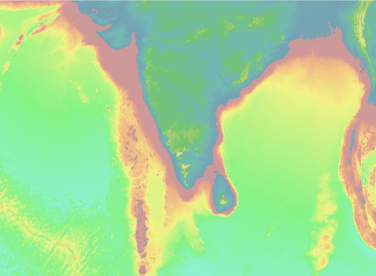
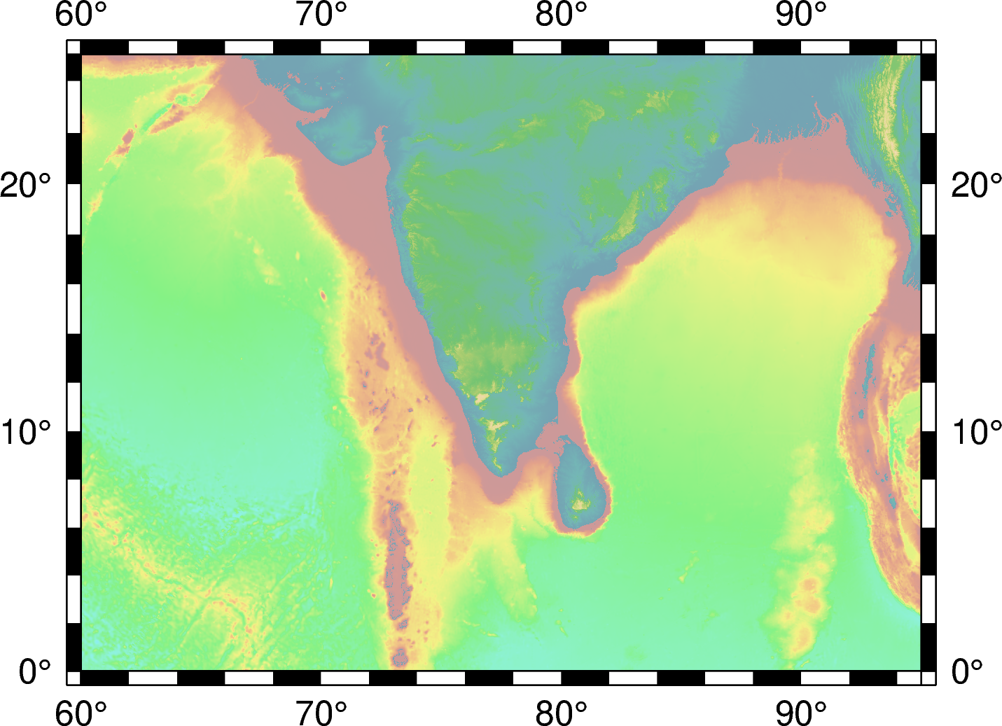
In this post, we will demonstrate the PyGMT implementation by plotting the topographic map of southern India. We will also plot some markers on the map.

Importing Libraries

The first thing I like to do is to import all the necessary libraries for the task. This keeps the code organized.

import pygmt

minlon, maxlon = 60, 95
minlat, maxlat = 0, 25

Define topographic data source

The topographic data can be accessed from various sources. In this snippet below, I listed a couple of sources.

#define etopo data file
# topo_data = 'path_to_local_data_file'
topo_data = '@earth_relief_30s' #30 arc second global relief (SRTM15+V2.1 @ 1.0 km)
# topo_data = '@earth_relief_15s' #15 arc second global relief (SRTM15+V2.1)
# topo_data = '@earth_relief_03s' #3 arc second global relief (SRTM3S)

Initialize the pyGMT figure

Similar to the matplotlib’s fig = plt.Figure(), PyGMT begins with the creation of Figure instance.

# Visualization
fig = pygmt.Figure()

Define CPT file

# make color pallets
pygmt.makecpt(
    cmap='topo',
    series='-8000/8000/1000',
    continuous=True
)

Plot the high resolution topography from the data source

Now, we provide the topo_data, region and the projection for the figure to plot. The region can also be provided in the form of ISO country code strings, e.g. TW for Taiwan, IN for India, etc. For more ISO codes, check the wikipedia page here. In this example, we used the projection of M4i, which specifies four-inch wide Mercator projection. For more projection options, check here.

#plot high res topography
fig.grdimage(
    grid=topo_data,
    region=[minlon, maxlon, minlat, maxlat],
    projection='M4i'
    )

#plot high res topography
fig.grdimage(
    grid=topo_data,
    region=[minlon, maxlon, minlat, maxlat],
    projection='M4i',
    frame=True
    )

#plot high res topography
fig.grdimage(
    grid=topo_data,
    region=[minlon, maxlon, minlat, maxlat],
    projection='M4i',
    shading=True,
    frame=True
    )

Plot the coastlines/shorelines on the map

Figure.coast can be used to plot continents, shorelines, rivers, and borders on maps. For details, visit pygmt.Figure.coast.

fig.coast(
    region=[minlon, maxlon, minlat, maxlat],
    projection='M4i',
    shorelines=True,
    frame=True
    )

Plot the topographic contour lines

We can also plot the topographic contour lines to emphasize the change in topography. Here, I used the contour intervals of 4000 km and only show contours with elevation less than 0km.

fig.grdcontour(
    grid=topo_data,
    interval=4000,
    annotation="4000+f6p",
    limit="-8000/0",
    pen="a0.15p"
    )

Plot data on the topographic map

## Generate fake coordinates in the range for plotting
lons = minlon + np.random.rand(10)*(maxlon-minlon)
lats = minlat + np.random.rand(10)*(maxlat-minlat)

# plot data points
fig.plot(
    x=lons,
    y=lats,
    style='c0.1i',
    color='red',
    pen='black',
    label='something',
    )

We plot the locations by red cicles. You can change the markers to any other marker supported by GMT, for example a0.1i will produce stars of size 0.1 inches.

Plot colorbar for the topography

Default is horizontal colorbar

# Plot colorbar
fig.colorbar(
    frame='+l"Topography"'
    )

For vertical colorbar:

# For vertical colorbar
fig.colorbar(
frame='+l"Topography"',
position="x11.5c/6.6c+w6c+jTC+v"
)

We can define the location of the colorbar using the string x11.5c/6.6c+w6c+jTC+v. +v specifies the vertical colorbar.

Output the figure to a file

Similar to matplotlib, PyGMT shows the figure by

# save figure
fig.show() #fig.show(method='external')

To save figure to png. PyGMT crops the figure by default and has output figure resolution of 300 dpi for png and 720 dpi for pdf. There are several other output formats available as well.

# save figure
fig.savefig("topo-plot.png", crop=True, dpi=300, transparent=True)

fig.savefig("topo-plot.pdf", crop=True, dpi=720)

If you want to save all formats (e.g., pdf, eps, tif) then

allformat = 1

if allformat:
    fig.savefig("topo-plot.pdf", crop=True, dpi=720)
    fig.savefig("topo-plot.eps", crop=True, dpi=300)
    fig.savefig("topo-plot.tif", crop=True, dpi=300, anti_alias=True)

Complete Script

Plot Focal Mechanism on a Map

How would you plot the focal mechanism on a map? This can be simply done in GMT using the command psmeca. But PyGMT do not support psmeca so far. So, we use a workaround. We call the GMT module using the PyGMT’s pygmt.clib.Session class. This we do using the context manager with in Python.

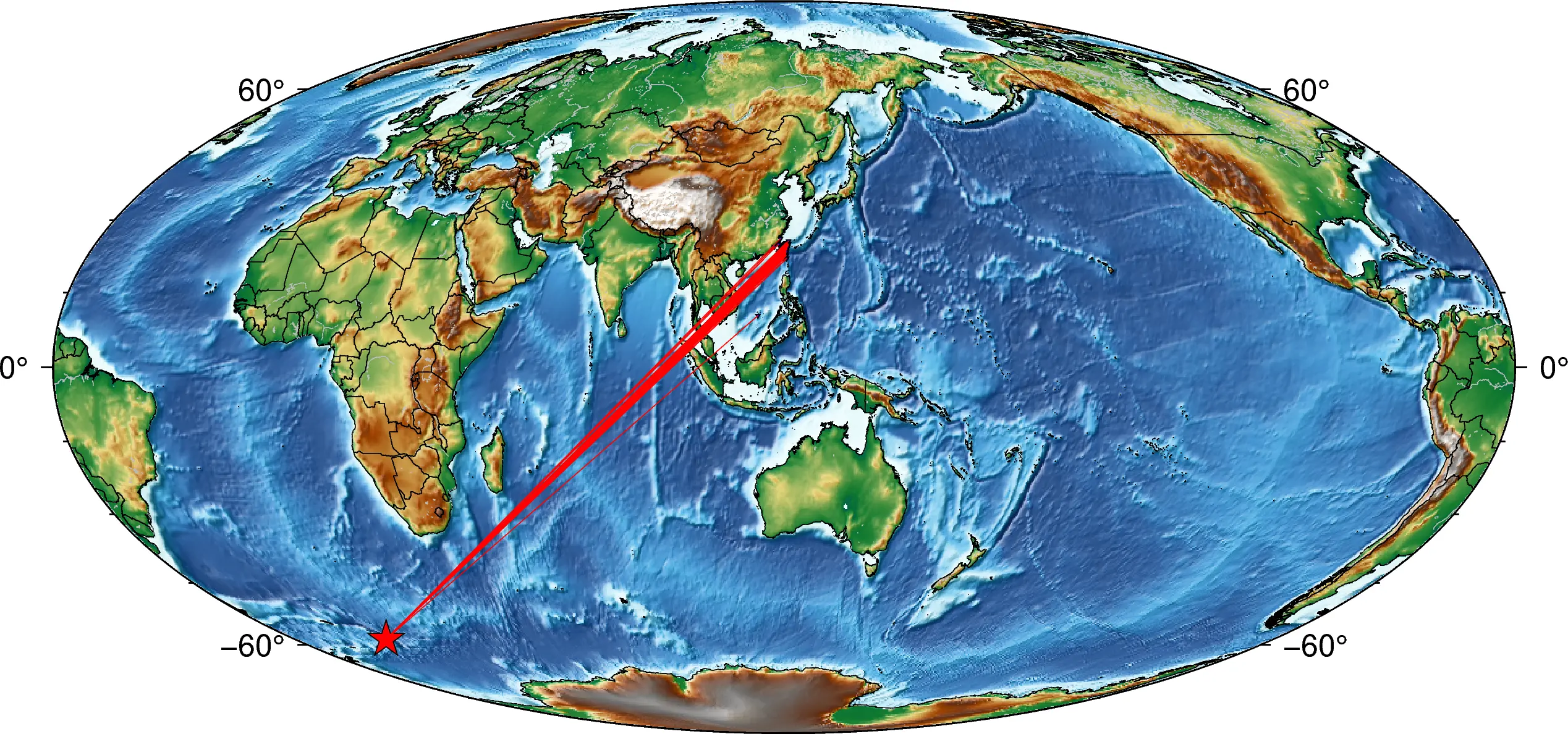
Plotting interstation paths between two stations

The following script uses the sel_pair_csv file for the coordinates of the pairs of stations. The sel_pair_csv file is a csv file that is formatted like:

   stn1     stlo1    stla1  stn2     stlo2    stla2
0  A002  121.4669  25.1258  B077  120.7874  23.8272
1  A002  121.4669  25.1258  B117  120.4684  24.1324
2  A002  121.4669  25.1258  B123  120.5516  24.0161
3  A002  121.4669  25.1258  B174  120.8055  24.2269
4  A002  121.4669  25.1258  B183  120.4163  23.8759

Event-Station Map

Here, I used the Mollweide projection but this code can be applied for any other projections with a little tweak.

The first few lines of the data file are:

References

1. Uieda, L., Wessel, P., 2019. PyGMT: Accessing the Generic Mapping Tools from Python. AGUFM 2019, NS21B--0813.
2. Wessel, P., Luis, J.F., Uieda, L., Scharroo, R., Wobbe, F., Smith, W.H.F., Tian, D., 2019. The Generic Mapping Tools Version 6. Geochemistry, Geophys. Geosystems 20, 5556–5564. https://doi.org/10.1029/2019GC008515