Efficiently compute spectrogram for large dataset in python

In previous posts, we have obtained the spectrogram of time series (seismic or otherwise) using mainly two approaches. We first used the Obspy’s spectrogram method to plot the spectrogram for seismic time series (see post 1 and post 2). We have then modified the Obspy’s spectrogram method to customize it to work more efficiently for our purpose (see post). We have also used MATLAB to plot the spectrogram (see here). But for most of the methods we used, we have seen that they suffer to compute the spectrogram for larger time series data. In this post, we will explore another module to compute the spectrogram of the time series.

Librosa

Librosa is a Python package designed for music and audio signal analysis. However, we will explore it for analyzing the seismic time series. This package has been designed for the purpose of applying machine learning analysis on the music data. For this sake, the package is required to be very efficient.

Librosa’s spectrogram operations include the short-time Fourier trans- form (stft), inverse STFT (istft), and instantaneous frequency spectrogram (ifgram), which provide much of the core functionality for down-stream feature analysis (see 1). Additionally, an efficient constant-Q transform (cqt) implementa- tion based upon the recursive downsampling method of Schoerkhuber and Klapuri [Schoerkhuber10] is provided, which produces logarithmically-spaced frequency representations suitable for pitch-based signal analysis. Finally, logamplitude provides a flexible and robust implementation of log-amplitude scaling, which can be used to avoid numerical underflow and set an adaptive noise floor when converting from linear amplitude. For details, check the references.

For spectrogram analysis, Librosa stores the spectrograms are stored as 2-dimensional numpy arrays, where the first axis is frequency, and the second axis is time.

Parameters used by Librosa

Some of the parameters used by the Librosa for analysis:

sr = sampling rate (Hz), default: 22050
frame = short audio clip
n_fft = samples per frame, default: 2048
hop_ length = # samples between frames, default: 512

Spectral analysis using Librosa

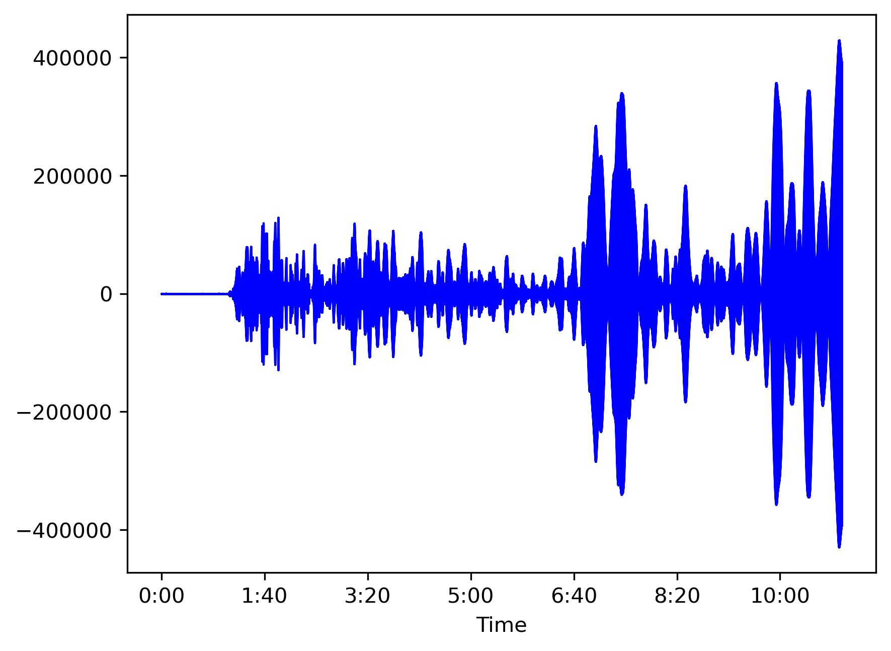
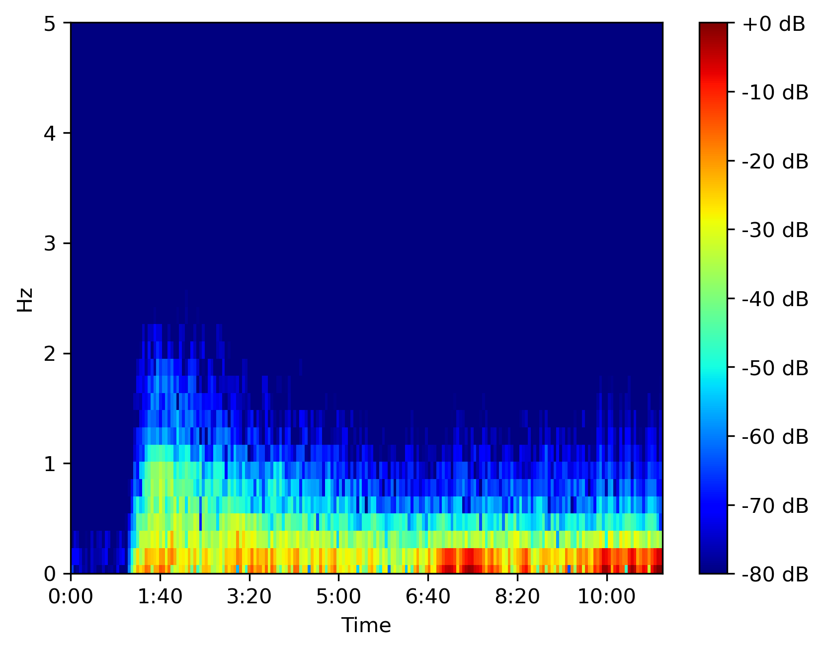
Let us select an event: 2021-07-29 Mww8.2 Alaska Peninsula, and a station to look at the waveforms: PFO: Pinon Flat, California, USA. The data is raw and downloaded from IRIS.

Plot waveforms

from obspy import read
import librosa
import librosa.display
import matplotlib.pyplot as plt
import numpy as np

dataFile = '2021-07-29-mww82-alaska-peninsula-2.miniseed'

st0 = read(dataFile)
st = st0.select(channel='BHZ', location='00')
print(st)

# play with hop_length and nfft values
hop_length = 128
n_fft = 256
cmap = 'jet'
bins_per_octave = 12
auto_aspect = False
y_axis = "linear"  # linear or log
fmin = None
fmax = 5.0

data = st[0].data.astype('float32')
sr = int(st[0].stats.sampling_rate)
max_points = int(st[0].stats.npts)
offset = 0

# Waveplot
fig, ax = plt.subplots()
librosa.display.waveshow(data, sr=sr, max_points=max_points,
                         x_axis='time', offset=offset, color='b', ax=ax)
plt.savefig('waveplot.png', bbox_inches='tight', dpi=300)
plt.close()

Plot spectrogram

# Librosa spectrogram
D = librosa.amplitude_to_db(
    np.abs(librosa.stft(data, hop_length=hop_length, n_fft=n_fft)), ref=np.max)


fig, ax = plt.subplots()

img = librosa.display.specshow(D, y_axis=y_axis, sr=sr,
                               hop_length=hop_length, x_axis='time', ax=ax, cmap=cmap, bins_per_octave=bins_per_octave,
                               auto_aspect=auto_aspect)

if fmin is not None:
    fmin0 = fmin
else:
    fmin0 = 0

if fmax is not None:
    fmax0 = fmax
else:
    fmax0 = sr/2

ax.set_ylim([fmin, fmax])
fig.colorbar(img, ax=ax, format="%+2.f dB")
plt.savefig('spectrogram.png', bbox_inches='tight', dpi=300)
plt.close()

References

1. McFee, Brian, Colin Raffel, Dawen Liang, Daniel PW Ellis, Matt McVicar, Eric Battenberg, and Oriol Nieto. “librosa: Audio and music signal analysis in python.” In Proceedings of the 14th python in science conference, pp. 18-25. 2015.
2. Schoerkhuber, Christian, and Anssi Klapuri. Constant-Q transform toolbox for music processing. 7th Sound and Music Computing Conference, Barcelona, Spain. 2010.
3. Youtube Video Librosa Audio and Music Signal Analysis in Python Brian McFee