Transfer learning applied on the unsplash data using alexnet pretrained network (codes included)
Transfer learning using the pre-trained deep learning networks from MATLAB can be easily implemented to achieve fast and impressive results
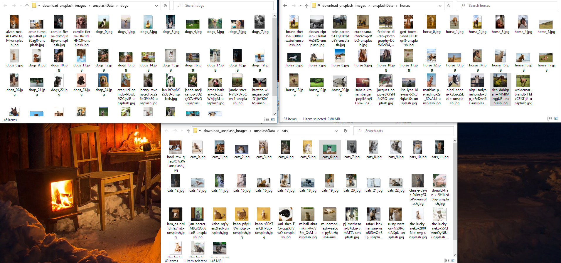
I obtained the image data from Unsplash. I downloaded 42 cats images, 46 dogs images, and 35 horse images for the input into the pretrained Alexnet model in MATLAB. For details about the Alexnet network in MATLAB, see its documentation.
Similar posts
Alexnet
AlexNet is a convolutional neural network that is 8 layers deep. The MATLAB has a pretrained version of the network trained on more than a million images from the ImageNet database. The pretrained network can classify images into 1000 predefined object categories.
The training for the 1000 object categories on a million images has made the the network learn rich feature representations for a wide range of images.
Installation
You can check the installation of alexnet by typing
alexnet
at the command line. If its not installed then it will prompt a link to the required support package in the Add-On Explorer. Simply, follow the link.
Why Transfer Learning?
Transfer learning has become popular in deep learning applications because of its speed and easy implementation. One can take a pretrained network and use it as a starting point to learn a new task. This quickly transfer learned features to a new task using a smaller number of training images.
Data
I obtained the three categories of images from the Unsplash website. Unsplash provides millions of high-quality free images. I obtained the images for cats, dogs and horses. There is no specific reason for using these categories but using cats and dogs have become standard for testing any model as it provides sufficient robustness.
I saved the data into three subfolders folders labeled with cats, dogs, and horses under the folder unsplashData. I kept the zipped data into the folder containing the script.

cats, dogs, and horses obtained from unsplashAnalysis
Prepare data
The first thing we do it to unzip the data using the unzip command. Then we automatically labels the images based on folder names and stores the data as an ImageDatastore object.
clear; close; clc;

%% Unzip and load the new images as an image datastore
filename = 'unsplashData';
unzip(strcat(filename,'.zip'));

% imageDatastore automatically labels the images based on folder names and stores the data as an ImageDatastore object
imds = imageDatastore(filename, ...
    'IncludeSubfolders',true, ...
    'LabelSource','foldernames');
Divide the data into training and validation data sets
We use 70% of the randomly selected images for training and 30% for validation.
[imdsTrain,imdsValidation] = splitEachLabel(imds,0.7,'randomized');
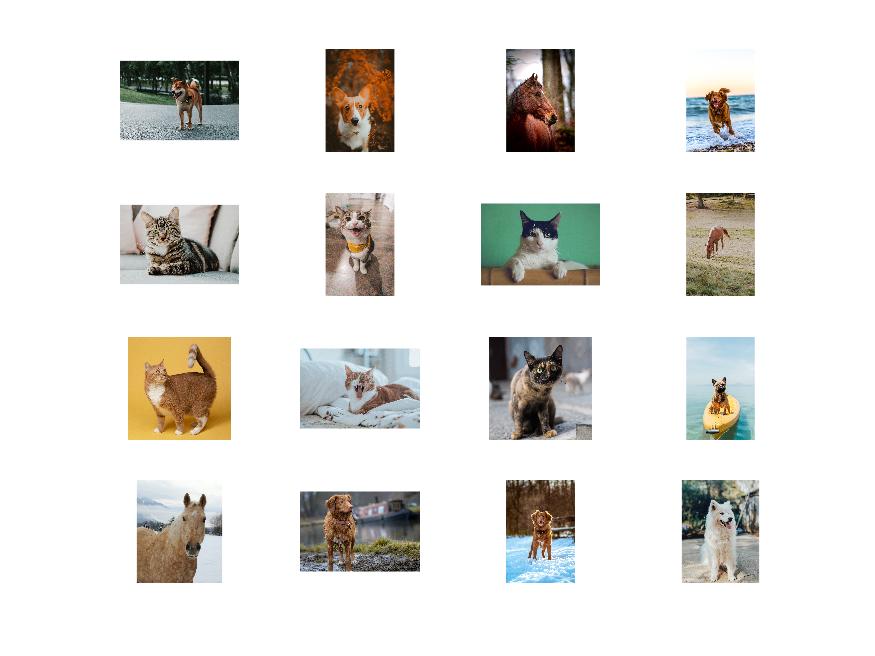
Visualize the loaded images
We plot the 16 randomly selected data.
visualize = 1;
if visualize==1
    numTrainImages = numel(imdsTrain.Labels);
    idx = randperm(numTrainImages,16);
    fig1 = figure;
    for i = 1:16
        subplot(4,4,i)
        I = readimage(imdsTrain,idx(i));
        imshow(I)
    end
    print(fig1,strcat(filename,'input-data-selected'),'-djpeg')
end

Load Pretrained Network
net = alexnet;
inputSize = net.Layers(1).InputSize
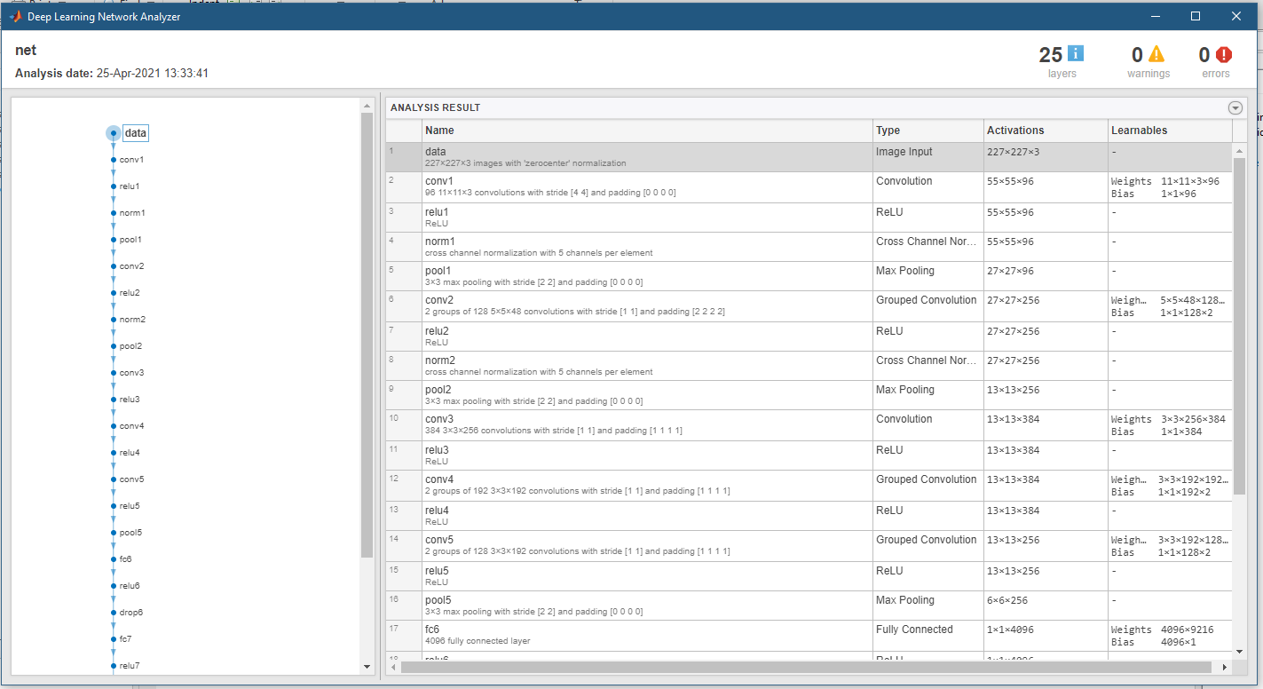
To analyze the layers of the alexnet network.
inspect_network=0;
if inspect_network==1
    analyzeNetwork(net)
end

Replace the final three layers
We extract all layers, except the last three, from the pretrained network. One can increase the WeightLearnRateFactor and BiasLearnRateFactor values of the fully connected layer to learn faster in the new layers than in the transferred layers
layersTransfer = net.Layers(1:end-3);

numClasses = numel(categories(imdsTrain.Labels)) %the number of classes in the new data

layers = [
    layersTransfer
    fullyConnectedLayer(numClasses,'WeightLearnRateFactor',20,'BiasLearnRateFactor',20)
    softmaxLayer
    classificationLayer];
Use an augmented image datastore to automatically resize the training images
The alexnet network has been designed to work on the images of fixed dimension (227-by-227-by-3). We follow the standard operations to augment the training images - randomly flip the training images along the vertical axis, randomly translate them up to 30 pixels horizontally and vertically. Data augmentation is necessary to prevent the network from overfitting and memorizing the exact details of the training images.
pixelRange = [-30 30];
imageAugmenter = imageDataAugmenter( ...
    'RandXReflection',true, ... %randomly flip the training images along the vertical axis
    'RandXTranslation',pixelRange, ... %randomly translate them up to 30 pixels horizontally and vertically
    'RandYTranslation',pixelRange);


augimdsTrain = augmentedImageDatastore(inputSize(1:2),imdsTrain, ...
    'DataAugmentation',imageAugmenter);

% automatically resize the validation images without performing further data augmentation
augimdsValidation = augmentedImageDatastore(inputSize(1:2),imdsValidation);
Fine tune the training options
The goal of applying transfer learning is to keep the features from the early layers of the pretrained network (the transferred layer weights).
options = trainingOptions('sgdm', ...
    'MiniBatchSize',10, ... %when performing transfer learning, you do not need to train for as many epochs
    'MaxEpochs',6, ...
    'InitialLearnRate',1e-4, ... %slow down learning in the transferred layers ( fast learning only in the new layers and slower learning in the other layers)
    'Shuffle','every-epoch', ...
    'ValidationData',augimdsValidation, ...
    'ValidationFrequency',3, ...
    'Verbose',false, ...
    'Plots','training-progress', ...
    'ExecutionEnvironment','auto'); %Hardware resource for training network - auto, cpu, gpu, multi-gpu, parallel
Train the network
We train the network consisting of the transferred and new layers.
netTransfer = trainNetwork(augimdsTrain,layers,options); %By default, trainNetwork uses a GPU if one is available
Classify Validation Images
[YPred,scores] = classify(netTransfer,augimdsValidation); %classify using the fine-tuned network
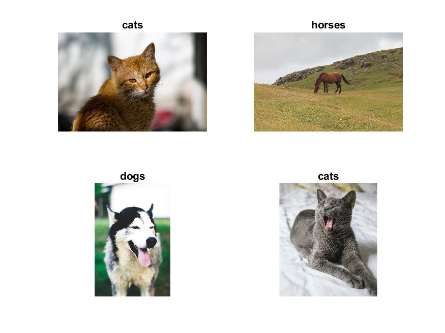
We display four sample validation images with their predicted labels.
classify_visualize = 1;
if classify_visualize==1
    idx = randperm(numel(imdsValidation.Files),4);
    fig = figure;
    for i = 1:4
        subplot(2,2,i)
        I = readimage(imdsValidation,idx(i));
        imshow(I)
        label = YPred(idx(i));
        title(string(label));
    end
    print(fig,strcat(filename,'classification-result'),'-djpeg')
end

Classification accuracy
Classification accuracy gives the fraction of labels that the network predicts correctly.
YValidation = imdsValidation.Labels;
accuracy = mean(YPred == YValidation)
accuracy =

    0.9189
Please note that we used the accuracy metric for classification because our target classes are well-balanced. We have roughly the same number of cats, dogs and horses images.
Conclusions
I used the pre-trained Alexnet network from MATLAB to fine-tune it with the Unsplash data. However, it has the potential for any classification problems with the image data. We should also explore several other pre-trained networks provided by MATLAB such as squeezenet, resnet18, googlenet, etc to achieve better accuracy. The accuracy depends highly on the data quantity, quality, and model parameters such as the number of layers.
Complete Code
Disclaimer of liability
The information provided by the Earth Inversion is made available for educational purposes only.
Whilst we endeavor to keep the information up-to-date and correct. Earth Inversion makes no representations or warranties of any kind, express or implied about the completeness, accuracy, reliability, suitability or availability with respect to the website or the information, products, services or related graphics content on the website for any purpose.
UNDER NO CIRCUMSTANCE SHALL WE HAVE ANY LIABILITY TO YOU FOR ANY LOSS OR DAMAGE OF ANY KIND INCURRED AS A RESULT OF THE USE OF THE SITE OR RELIANCE ON ANY INFORMATION PROVIDED ON THE SITE. ANY RELIANCE YOU PLACED ON SUCH MATERIAL IS THEREFORE STRICTLY AT YOUR OWN RISK.